The Testing Column: Equating the MBE

This article originally appeared in The Bar Examiner print edition, September 2015 (Vol. 84, No. 3), pp 29–36.

By Mark A. Albanese, PhDEquating is the most complex process underlying the production of scores for the MBE. Explaining it to people is the quickest way to end a party, yet it is still the topic I am most frequently questioned about. I am not the first NCBE Director of Testing to have experienced this. In fact, this column and other articles in the Bar Examiner have addressed the topic of equating several times over the years. They say that doing the same thing over and over again and each time expecting a different outcome is a sign of insanity. The fact that I am writing this article makes me a little worried about myself, but here goes.

The only constant is change. In the high-stakes testing world, we have to change almost everything each time we administer a test. Because the stakes are high for the bar examination, there are any number of examinees who would dearly love to see items on the MBE before the test is administered. Thus, we wait for a few administrations before we reuse any question, or item, and we use any given item for only a few test administrations before we quit using it forever. Against this backdrop, we also have to ensure that a score we produce retains its meaning across time and space. A score earned in 2013 in New York should have the same meaning as a score earned in 2014 in Guam. We rely on standardized administration of the MBE to ensure that where an examinee sits for the exam (space) does not affect his or her score. To ensure that whether an examinee takes the MBE in 2009 or 2015 or July or February (time) is not a factor, we rely upon equating.

Each time NCBE builds an MBE test, we do our best to choose items that will work the same way as items have in the past. The exam is built according to a detailed subject matter blueprint and statistical criteria that ensure comparability of what is measured across time. (One recent update is the addition of Civil Procedure to the February 2015 MBE, which was a change in content that will continue going forward.) However, with so many items and so much content to cover, it is nearly impossible to build a test that has exactly the same level of difficulty as those previously administered. The overall difficulty of an examination will be slightly different each time. Equating is the process of statistically adjusting scores to account for these differences in difficulty.

In this article, I will describe the process we use at NCBE to develop the MBE so that it can be equated, as well as the process we use in scaling and equating the examination. By necessity, my article is an oversimplification of the actual processes we use, but I hope that it will give you a sense of what we do.

Equating Overview

The purpose of equating is to adjust for any change in the difficulty of a newly created examination so that the exam’s scores are comparable to the scores of previous exams. To do this, there must be something about the new exam that remains constant or at least has links to past examinations. There are many ways this can be achieved, but the way we achieve it with the MBE, and an approach that is com­monly used in other high-stakes testing programs, is to embed a mini-MBE within each test we administer that consists of previously used items. The items on the mini-MBE are chosen so that they represent as closely as possible the content of the overall examination. The items on the mini-MBE are called the equators, because, as you might guess, they are used to equate the examination. Because the equators have been used previously, we know approximately the percentage of examinees who will answer them correctly (difficulty1) and how much more likely it is that they will be answered correctly by examinees who do well on the overall test than by those who do not (discrimination2). This statistical information gives us the ability to link performance on the current examination to previous examinations. If examinees on the current test perform more poorly on the equator items than those who took the examination previously (as was the case in July 2014), we can attribute examinee performance differences on the equators to differences in the examinees themselves, because the equator items are unchanged. We then use a statistical adjustment to make the performance on the rest of the items conform to that of the equator items. I will return to this later to show how this works.

Equator Item Selection

As a set, equators are intended to comprise a mini-exam that is representative of a full MBE from both a subject-area and a statistical perspective. All equators have been used as scored items on at least one previous MBE administration.

Equator sets must satisfy specific psychometric criteria. When selecting an equator set, both ­within each subject area and as a complete set, various aspects of the potential items are considered, including the following:

1. Date of most recent use. Equators are selected from numerous past administrations. One-half of an equator set should have appeared most recently on a February administration, and the other half on a July administration.
2. Placement from most recent use. One-half of an equator set should have appeared most recently on a morning test form, and the other half on an afternoon test form. All equators are placed in a position on the test form that is as close as possible to their placement in their most recent use.
3. Statistics from most recent use. An equator set should have an average overall difficulty that is representative of the average overall difficulty and discrimination that meets or exceeds specified criteria.
4. Content representation. The content assessed by the selected equators within each subject area should be representative of the spread of items within that subject area that will appear on the full exam.

An item selected as an equator is not edited from the version that appeared in its most recent use. This helps to ensure that equators perform as closely as possible to the way they performed previously.

Once equators are selected (see the article by C. Beth Hill for more information about this process), psychometric staff members review the set of items for compliance with established statistical criteria. As with most things in life, it is rare that you get to have your cake and eat it too. The same is true in the selection of equators. Equator selection requires a balance between the desire to meet statistical criteria and the desire for content representation and conforming to item-writing best practices (a combination of avoidance of known flaws in the construction of an item that can affect examinee performance combined with stylistic issues designed to provide clarity and avoid confusion). If necessary, items are replaced with other items that are subject to the same delicate balance of meeting the web of intersecting criteria for content, statistics, and best practices.

Scaling

Scaling is the method by which we assign numbers to something we measure. One of the most com­monly encountered examples of different scaling methods is that of temperature, which can be ­reported on the Fahrenheit or Celsius scale. Both scales are anchored to the freezing and boiling points of water (0 and 100 degrees Celsius, respectively; 32 and 212 degrees Fahrenheit, respectively). The Fahrenheit scale is more finely graded than the Celsius scale because there are 180 integer points between freezing and boiling as opposed to only 100 points on the Celsius scale. Is one better than the other? Not really; it is a matter of preference. The really important thing is not to mix them up. If you think you are jumping into a pool with 100-degree Fahrenheit water, you will be in for an unpleasant surprise if the ther­mostat is scaled in Celsius.

Typically, scaling in the testing context is designed so that examinees will not think their scaled score is either a number correct or a percent correct. The equating process makes adjustments in scores that can create a fair amount of confusion if examinees think their scaled score is the number correct or the percent correct. One of the goals, then, of scaling is to express scores in such a manner as to avoid that confusion. Therefore, clearly unique score values are typically chosen for a score scale. For example, the Scholastic Aptitude Test (SAT) scaled scores were originally set to have a minimum of 200 and a maximum of 800 with a mean set at 500 and a standard deviation of 100. Scores have migrated upward over the years as test takers have become better prepared, but the interpretation is still based on that original scale. (As a reminder, the mean is the sum of scores divided by the number of scores; the standard deviation can be thought of as the average deviation of scores from the mean, although its exact computation is more complex.)

For better or worse, the MBE scale we report appears to be based on the number of items an­s­­­wered correctly by examinees on the 200-item ­examination administered in July 1972 (the second-ever administration of the MBE). Even today, after 43 years, the scores from the MBE can be thought to be referenced to that early examination. It is not a direct link, however. Not one item on today’s examination or probably any examination since 1980 was on the test administered in 1972. The relationship is through the equatings that have occurred since that time.

Each equating links scores to at least two earlier exams, one or more in July, the other(s) in February. Because all of these exams have been equated to earlier examinations, there is an unbroken chain of linkages back to that 1972 examination. Because the test changes its character over time and the linkages become more fragile as time passes, the base test used to serve as the reference for computing statistics employed in scaling is reset periodically. Our current base is the July 2001 examination. The difference is primarily statistical. Conceptually, the scale still harkens back to the July 1972 examination.

Equating

The driving force in how we equate the MBE is performance on the equator items. We first assess whether what I refer to as the genetic makeup of our equators has changed. The genetic makeup of an item consists of its discrimination, difficulty, and guessing parameters, as described later. While evolution may have benefited our ancestors, it is not something we want to see in equators. If the genetic makeup of an item has changed, we remove the item from the equating set and treat it like the rest of the items on the test. In any given administration, very few items show evolutionary tendencies such that they have to be removed from the equator item set.

After completing our analysis of the stability of the equators’ genetics, we evaluate the equators’ performance. If the performance on the equator items in their current administration is lower than in their previous administration, we conclude that the present examinees are not as proficient as the previous examinees. If performance on the equator items is higher, we conclude that the present examinees are more proficient than the previous examinees. We then need to adjust scores on the total set of items to proportionately reflect that conclusion.

The simplest adjustment would be to obtain the difference in average difficulty for the equator items in the current administration versus the previous administration and apply that difference to the items that were non-equators. So, if the average difficulty on the equators was 5% lower in the present administration (the difficulty value expressing the percentage of examinees who answered the items correctly—therefore a 5% lower value indicating that fewer examinees answered the items correctly), then the performance on the other items would also be lower in the present administration, compared with the expected performance had those items been answered by the previous group of examinees. Therefore, we would add 5% to the score on the non-equator items before combining the equator and non-equator scores and referencing the total score to the raw-to-scaled-score conversion chart from the previous administration.3 (After the equating process for each administration, a raw-to-scaled-score conversion chart is produced to relate the raw scores to scaled scores.)

While adjusting scores on the basis of the average difficulty of the equator items would be the easiest approach, it assumes that the differences in the equator scores project equally for all examinees at all points of the score range. However, that is not how it usually works. Usually the relationship is proportionate to an examinee’s score, so lower-performing examinees are affected less than higher-performing examinees. Thus, the mathematical relationship may be better modeled, for example, by assuming that there is a linear relationship between the current and past performances on the equator items and that this relationship then extends to the non-­equator items used to compute a score.4 With a linear approach, it is not just a value like the mean that is added or subtracted from scores, but there is a slope (change in current scores divided by the change in scores from previous use) that scores are multiplied by. The slope that scores get multiplied by and the value that is then added to scores is first derived for the equators and then applied to the rest of the items similar to the process described above for the mean. However, this is just getting you primed for the real thing, because when we adjust MBE scores at NCBE, we do not use either of these approaches, but one based upon Item-Response Theory (IRT).

Item-Response Theory

IRT Background

Prior to the advent and implementation of IRT, the statistics used for test development relied almost exclusively on the two types of item statistics that I introduced earlier: the percentage of examinees who answered an item correctly (difficulty) and how well the item differentiated between examinees who did well on the overall examination and those who did not (discrimination). The problem with these statistics is that they are dependent upon the examinees used in their computation being comparable to examinees in the future. To the extent that future examinees are not comparable to those for which an item’s statistics were obtained, the results for that item will not conform to what is expected (i.e., have the same difficulty relative to the other items, correlate the same with the other items and with the test as a whole, etc.).

For the MBE, this is a particular problem, because the February examinee population is composed of approximately 60% retakers compared to less than 20% in July. Retakers are generally known to perform less well, on average, than first-time takers, and we consistently find that the performance of February MBE takers is lower than that of July MBE takers. When we compare the percent correct for an item that was previously administered in July with its performance when it was previously administered in February, the July percent correct is often 5–10% higher than that obtained in February. IRT has properties that overcome the differences in February and July examinees.

IRT Concepts

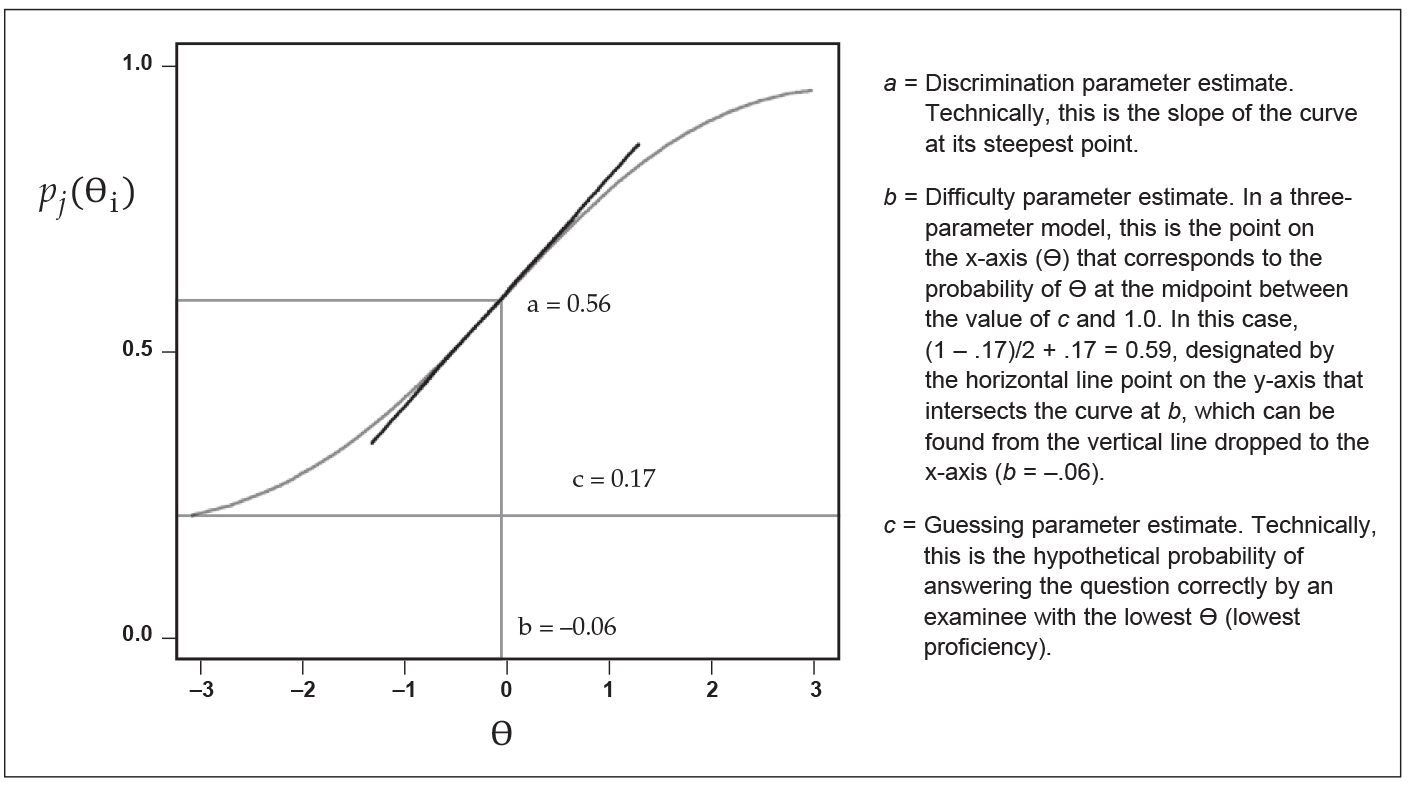
The basic concepts of IRT were developed as long ago as the 1950s, but they did not become practical for use in actual tests until the 1980s and 1990s when computing power became adequate to do the required analyses.5 In a way, you can think of IRT as deciphering an item’s DNA, and just as human DNA is sometimes used to predict human tendencies, the IRT DNA code is used to describe an item’s tendencies. In the world of IRT, there are different models that are used relatively interchangeably. The one we use is called the three-parameter model, named as such because it has three components (called parameters), which I am likening to an item’s DNA. The three parameters comprising the item’s DNA are creatively named a, b, and c. The item parameters are defined by a mathematical model that relates them to a parameter reflecting an examinee’s overall test performance, designated by the Greek letter theta (Ɵ). These theoretical parameters are grounded in the reality of test performance by the following relationships: a is related to the discrimination of the item; b is related to the difficulty of the item; c is related to the amount of guessing on the item; and Ɵ, as noted above, is related to the examinee’s proficiency as reflected in his or her performance on the entire test.

The mathematical model that relates them all together is as follows:

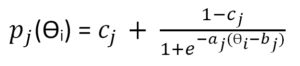
where p_j(Ɵ_i) refers to the probability of ­correctly answering any particular item (designated by j) for a person (designated by i) with a given value of Ɵ_i and e represents a constant that is the base of the natural logarithm and is approximately equal to 2.71828.

Figure 1 shows how a, b, and c interrelate in a plot of p_j(Ɵ_i) versus Ɵ. What is most important to remember for the remainder of this discussion is that each item has its own set of parameter estimates a, b, and c, and each examinee has a value relating to proficiency as reflected in his or her performance on the entire test that is designated by Ɵ.

Figure 1: Example of a plot showing the probability of answering an item correctly as a function of examinee proficiency

IRT Equating Process

The actual IRT equating process is the subject of entire books, and I cannot hope to do it justice in a few paragraphs.6 What I hope to do is give you an overview of the mechanics of what happens using my DNA metaphor. My goal is to give you a general understanding of the process and confidence in its results.

The first step in the equating process for an examination is to obtain the estimates of each item’s DNA parameters a, b, and c. This is done by a process called item calibration. I won’t bore you with the details, but it is a computationally intense statistical estimation process that simultaneously considers all parameters and makes incremental changes in each until stable estimates are achieved, a state called convergence. As you may be able to imagine, with 200 items and over 20,000 examinees in February and over 50,000 examinees in July, this is not something that can be done with a pad of paper and a pencil; the process relies on software programs specifically designed for such a statistical estimation process. Once we have estimates of a, b, and c and each person’s Ɵ values, we have some preliminary characteristics of items that are consistent within the current data; however, the items have no linkage to the historical genetics of the items.

The next step is where the equating and scaling process occurs. While there are different approaches that can be used to establish the linkage to a test’s historical roots, the particular one we use is called the Stocking-Lord method, named as such after its originators. The equator items now have two sets of parameter estimates, those from the current examination and those from previous use. From the two sets of equator item parameter estimates, two sets of Ɵ values are produced for each examinee. The set of item parameter estimates from previous use have historical item genetics that reach back to the July 1972 examination. The set of parameter estimates from the current administration have no such linkage. What both sets of estimates do have in common is the examinee’s proficiency as reflected in his or her performance on the entire test. So, the goal of this step is to find adjustments to the item parameter estimates for the current administration such that the Ɵ values generated have a relationship that is as close as possible to that for the Ɵ values generated from previous use. The mathematics behind the process again gets complex, but the process of getting to the item parameter adjustments is again incremental, as it was for obtaining the initial item parameter estimates during the calibration process referred to above. The item parameter estimates are adjusted one by one, and a statistic measuring the difference in the relationships between the new and old Ɵs and raw scores is computed. If the statistic indicates that the two are within a specified tolerance, the process is said to achieve convergence. If not, then a new value for another parameter is inserted and the process repeats until convergence is reached. This process eventually results in adjustments to each of the item parameters that will link them back to previous history in the same way that the previous item parameter estimates have been linked. As with the calibration process, with so many items and examinees and the demanding criteria that are used to define convergence, we can feel confident that what we have is something that is substantive and will stand the test of time.

The next step is to apply the item parameter equating adjustments to the rest of the items on the test. The final step is to produce a table that relates the raw scores to scaled scores.

Because of the equating and scaling process, these scaled scores have constant meaning and link back through their IRT genetics to all such scores that came before.

Final Comments

At present, we have two (or more) psychometricians independently do the equating using different programs at each examination. We have yet to have the separate results differ beyond more than two decimal places. If we ever do have differences between the different psychometricians’ results, we would achieve resolution to the differences before we would release scores.

The equating process has proven to be quite robust, meaning stable in the face of change. When we added Civil Procedure to the MBE in February 2015, we conducted the equating with and without the new Civil Procedure items. The mean of resulting scaled scores including the Civil Procedure items was 136.1696 versus 136.1766 without the Civil Procedure items. In the score range between 125 and 150—4 points below and 5 points above, respec­tively, where any jurisdiction sets its passing score—no examinee had scaled scores that made a practical difference.

In closing, I hope that this description of the equating we do for the MBE at least gives you confidence that the scaled scores we produce are based upon substance and the highest-quality methods.

Contact us to request a pdf file of the original article as it appeared in the print edition.

References

- Deborah J. Harris, Equating the Multistate Bar Examination, 72(3) The Bar Examiner 12–18 (August 2003).
- Michael T. Kane, Ph.D. & Andrew Mroch, Equating the MBE, 74(3) The Bar Examiner 22–27 (August 2005).
- Michael J. Kolen & Robert L. Brennan, Test Equating, Scaling, and Linking: Methods and Practices (Springer 3rd ed. 2014).
- Julia C. Lenel, Ph.D., Issues in Equating and Combining MBE and Essay Scores, (61)2 The Bar Examiner 6–20 (May 1992).
- Lee Schroeder, Ph.D., Scoring Examinations: Equating and Scaling, 69(1) The Bar Examiner 6–9 (February 2000).
- M.L. Stocking & F.M. Lord, Developing a Common Metric in Item Response Theory, 7 Applied Psychological Measurement 201–210 (1983).
Notes
- Item difficulty is the percentage of examinees who answered an item correctly. It is computed by taking the number of examinees who answer an item correctly and dividing by the total number of examinees and multiplying by 100. Sometimes it is left as a fraction and not multiplied by 100. Low values—for instance, 10 examinees answering an item correctly out of 100 taking the test, resulting in a difficulty of 10%—indicate that few examinees answered the item correctly, so the item is very difficult. High values—for instance, 90 examinees answering an item correctly out of 100 taking the test, resulting in a difficulty of 90%—indicate that a large number of examinees answered the item correctly, so the item is relatively easy. The term difficulty is something of a misnomer, because a high value means that an item is easy, while a low value indicates that an item is challenging. (Go back)
- The process for calculating an item’s discrimination can be thought of as taking the top quarter of examinees (for arcane psychometric reasons we actually use 27%) based upon total exam performance and putting them in a high box, and taking the lowest quarter of examinees based upon total exam performance and putting them in a low box. For examinees in the two boxes, we compute the percentage of examinees who answered the item correctly. The difference between the percentage in the high box and the percentage in the low box is the item discrimination. For example, say we have 100 examinees. Based upon the total score on a test, we put the top-scoring 25 in the high box and we put the lowest-scoring 25 in the low box. For item 1, say 20 of the 25 examinees in the high box answered the item correctly (80%) and 10 of the 25 examinees in the low box answered the item correctly (40%). Since discrimination indexes are usually reported as proportions, the discrimination would be 20/25 – 10/25 = .80 – .40 = .40. For item selection purposes, it is essential that the discrimination index be at least positive, if not greater than .20. (Go back)
- See Lenel 1992 for a more detailed example of how this is done. (Go back)
- See Harris 2003 for a more detailed example of how this is done. (Go back)
- See Harris 2003 and Kane & Mroch 2005; both describe IRT in different ways, and I encourage you to read these articles if my approach leaves you either wanting or wanting more. (Go back)
- See, e.g., Kolen & Brennan 2014. (Go back)
Mark A. Albanese, PhD, is the Director of Testing and Research for the National Conference of Bar Examiners.